A Beginner Guide To Logistic Regression In Python

Objective- Learn about the logistic regression in python and build the real-world logistic regression models to solve real problems.

Logistic regression modeling is a part of a supervised learning algorithm where we do the classification. Classification basically solves the world’s 70% of the problem in the data science division. And logistic regression is one of the best algorithms for the classification problem.

The real-time example can be-

• The bank may want to identify whether the loan will default or not
• A hyperlocal store may want to predict if they will have profit or loss on certain day or item
• Identifying if an email is spam or not
• A student may want to know if they will be getting the admission in their dream college or not and many more.

If you may have noticed here, I have only included the example where the answer is either yes/no or true/false or 1/0. And yes, that is the requirement for logistic regression.

When we can use logistic regression

The very first condition for logistic regression in python is, the response variable (or dependent variable) should be a categorical variable. And that too binomial categorical variable. That means it should have only two values- 1/0

Even if it has two value but in the form of Yes/No or True/False, we should first convert that in 1/0 form and then start with creating logistic regression in python.

What is a logistic regression model

The logistic regression model is one of the simplest machine learning models which is used for classification. And that too only for two-class classification. If your response variable has more than 2 options like grading system (where we can more than 2 grades) then we can’t apply logistic regression. In such case, Random forest algorithm in python or decision tree algorithm in python is recommended.

Logistic regression in python is quite easy to implement and is a starting point for any binary classification problem. It helps to create the relationship between a binary categorical dependent variable with the independent variables.

In this logistic regression using Python tutorial, we are going to read the following-

1. Logistic regression introduction
2. Linear regression vs logistic regression
3. Derive logistic regression mathematically
4. Creating a logistic regression model in python
5. Testing (doing prediction) the developed logistic regression model
6. Confusion Matrix to find the accuracy
7. ROC Curve to analyze the model
8. Summary of the developed model

Introduction to logistic regression

As said above, logistic regression is majorly used for predicting the binary categorical variable. Means those response variables which has only 2 options. This can be used to identify whether the person is diabetic or not and similar cause.

If you are continuous or discrete data and looking to do prediction, you may apply linear regression or similar.

And if you have categorical data but more than two class, you may apply a decision tree or random forest algorithms.

So, we can say that logistic regression is a special case of a linear regression model where the response variable is binomial categorical.

Linear regression vs logistic regression

The major difference between linear and logistic regression is the kind of variable these are being applied to. Linear regression is for discrete data whereas Logistic regression is for the categorical data.

Being said that, the predicted value for linear regression can be anything in the finite space. For example, let’s say we are working on a retail data to predict the profit. And so, the profit can be anything like- 100, 200, -150, 400, 345, etc.

And so, if we draw the graph for this, it can be somehow like this-

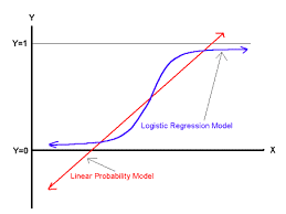
But as the predicted value of the logistic regression can be only 0 and 1 and so, the graph will be always between 0 and 1. As said earlier, logistic regression is just derived from linear regression only. In linear regression, we use ordinary least square (OLS) while in logistic regression, we use maximum likelihood estimation (MLE).

Sigmoid Function

We use the sigmoid function to manipulate the output between 0 and 1. The sigmoid function is also called a logistic function which provides S-shape curve and maps any real-value number between 0 and 1.

And so, if the output of the sigmoid function will be is more than 0.5, we can classify that to be 1 while if it is less than 0.5, it can be classified as 0.

For example, if the output of the sigmoid function is 0.7 then we can classify it as 1 while if it is 0.2 then we can classify it as 0. The sigmoid function is as below-

And so, the graph for the output of the sigmoid function will be like-

Now, let’s say we have two output of sigmoid function as 0.6 and 0.9. Now when we will take that to 0 or 1 then both will be converted to 1.

But the error associated with 0.6 predictions will be way more than 0.9. And that is the reason we always aim for the sigmoid output either near to 0 or near to 1 so that error will be less. And so, depending on how the accuracy of the model you are getting, the graph can vary like below-

As we can see, the more sigmoid output we will receive near to 0 and 1, the better curve we can get (ideal is the red line). The area below the curve is called as AUC (area under the curve) and explain the explanation of the covered data. And this curve is called the ROC curve which is the performance measurement parameter for logistic regression in python.

Derive logistic regression mathematically

Now let’s see how to derive the logistic regression model mathematically-

P(Y=1|X) is the probability that Y=1 given some value for X. Y can take only 2 values- 0 or 1.

For calculation, let’s write

P(Y=1|X) as p(x)

Here the right side is just the same equation for linear equation.

ln(p/1-p) = is known as “log-odds” or “odds ratio” or “logit” function.

How to create a logistic regression model in python using student dataset

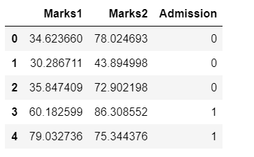
Now let’s start and see how to create logistic regression in python using a student dataset. The dataset can be downloaded from here and it has just three column-

1. Marks1- Marks of the student in the 1st subject
2. Marks2- Marks of the student in the 2nd subject
3. Admission- Response variable which has value either 0 or 1. 1 means the student will get admission and 0 means no admission.

I am going to do this in Jupyter notebook and you can do the same. If you are not aware of this, please install Anaconda where you will get Jupyter notebook including various tools. There are only the following steps in creating any machine learning model-

• Initialize the libraries and load the dataset
• EDA and data cleaning/preparation
• Split the dataset into test and train
• Create the model
• Do the prediction
• Check the accuracy and analyze the model

If looking for more free dataset, please check this post.

Initialize the required python libraries

We may need the following libraries- Pandas, sklearn, numpy, matplotlib, and seaborn. Let’s initialize these libraries so that we can work smoothly.

#import required libraries

#for data import and basic oprtaion
import pandas as pd
import numpy as np

#for visulization and plotting
import matplotlib.pyplot as plt
import seaborn as sns

#to view the plots in the jupyter notebook inline
%matplotlib inline

#to create the confusion matrix
from sklearn import metrics

#to split the dataset into train and test
from sklearn.model_selection import train_test_split
#or! Earlier train_test_split was in cross_validation
#from sklearn.cross_validation import train_test_split

#to apply logistic regresison
from sklearn.linear_model import LogisticRegression

Load the dataset and do an EDA

#load the dataset
data= pd.read_csv(r"C:\Users\Downloads\marks.csv")

Once the dataset is loaded, quickly use the head() to check the first five records-

#check top records
data.head()

Also, check for the null records. We can quickly look for the info() function which initially can tell us about non-null values:

#check info about the data
data.info()

This says we have a data frame which has 100 records and 3 columns. None of these columns are having any null values. Marks1 and Marks2 are float and Admission are of Integer datatype.

So, we are good on the EDA side and can go further.

Select the features

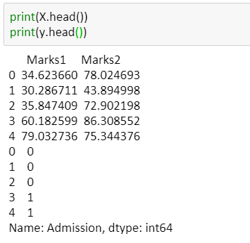
To apply the logistic regression, we provide two argument x and y. Where x represents all the independent variables and y represent the dependent variable. Let’s create x and y-

#split dataset in features and target variable
feature_cols = ['Marks1', 'Marks2']
X = data[feature_cols] # Features
y = data.Admission # Target variable

Split the dataset into test and train

We need basically two datasets one to develop the model and another to test our model for evaluating the performance.

We can use the function train_test_split() which is a part of sklearn library. This has majorly 4 argument-

1. Independent variable – X
2. Dependent variable- y
3. Test_size- This basically says the percentage of records we want to put in the test dataset. There is no specific rule on how much we should keep but ideally, it can be 40% or 30% or even 50%. This completely depends on the size of the dataset. If we have more samples, we can go ahead with more records in test dataset else less. As we just have 100 records in our dataset and so, let’s keep 25% records in test dataset and the remaining 75% in training dataset.
4. Random_state- to maintain the reproducibility of the random splitted data

#split the dataset in train and test
X_train,X_test,y_train,y_test=train_test_split(X,y,test_size=0.25,random_state=0)

X_train.shape

X_test.shape

Model Development

Now as we have splitted the dataset into train and test and so let’s start creating the logistic regression model in python on the training dataset.

To do that, we need to import the Logistic Regression module from sklearn.linear_model. And then need to create the logistic regression in python using LogisticRegression() function.

# instantiate the model using the default parameters
m1 = LogisticRegression()

# fit the model with data
m1.fit(X_train,y_train)

Do the prediction on the testing dataset

Now as we have created the model m1 on the testing dataset y_test. We can use the predict() function for the prediction on the test dataset. It takes the testing dataset (X_test in our case) as an argument.

#prediction on test dataset
y_pred=m1.predict(X_test)

y_test

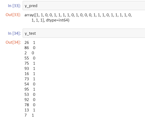This is the predicted values for the 25% data we kept in our testing dataset. That means the first two students will get the admission while the next two won’t and so on.

Let’s quickly print both the original test data prediction (y_test) and predicted values (y_pred) and match result.

As we can see, 1st four results are matching (just a coincidence ?). While for the 5th student we have predicted that the student will get admission while originally the dataset says, that 5th student won’t get admission. And so, this is a misclassification which is ean rror. Similarly, we can check for other records.

Definitely, we won’t be doing this manually and so, we have confusion matrix here.

Model Evaluation using Confusion Matrix

A confusion matrix is basically a two-way frequency table which is used to find the accuracy and error of the model. This tells about the number of correct and incorrect predictions for both 1 and o.

The confusion matrix shape will be like below-

Now let’s create the same for our model-

#confusion matrix
c1 = metrics.confusion_matrix(y_test, y_pred)
print(c1)

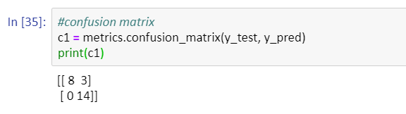This confusion matrix says-

• True positive (TP): 8 (We predicted admission and student got admission as well originally)
• True negative (TN): 14 (We predicted student won’t get admission and it originally also students didn’t get admission)
• False positive (FP): 0 (We predicted student will get admission but originally these students didn’t get admission)
• False negative (FN): 3 (We predicted student won’t get admission but originally these students didn’t get admission)

Accuracy = (TP+TN)/total

Accuracy= (8+14)/25= 22/25= 0.88= 88%

Error= (FP+FN)/total

Error= (3+0)/25= 3/25= 0.12= 12%

Now let’s look for the three model evaluation metrics-

• Accuracy- This is being given by the same confusion matrix which we drew above
• Precision- It’s about being precise! Means how accurate our model is
• Recall- Test for how correctly our model is able to predict that the students have got admission

#evaluation metrices
print("Accuracy:",metrics.accuracy_score(y_test, y_pred))
print("Precision:",metrics.precision_score(y_test, y_pred))
print("Recall:",metrics.recall_score(y_test, y_pred))

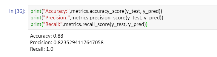So, we have 88% accuracy; 82% precision, and 100% recall.

AUC and ROC Curve

AUC (area under the curve) and ROC (Receiver Operating Characteristic) curve are also being used to evaluate the performance of the logistic regression we just created.

The ROC curve is being plotted between True positive rate (TPR) and False positive rate (FPR). These majorly comes from sensitivity and specificity.

#ROC curve and AUC value
y_pred_proba = m1.predict_proba(X_test)[::,1]
fpr, tpr, _ = metrics.roc_curve(y_test,  y_pred_proba)
auc = metrics.roc_auc_score(y_test, y_pred_proba)
plt.plot(fpr,tpr,label="data 1, auc="+str(auc))
plt.legend(loc=4)
plt.show()

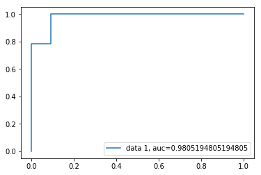This is the logistic regression curve we have received which is basically the ROC curve. The AUC value is 0.98 which is really great. An AUC value of 1 means a perfect classifier and 0,5 means worthless. Means we can say an AUC value of 0.5 is just a random prediction.

That’s all about the logistic regression in python. Our model is correctly able to predict 88 records out of 100 records which are decent.

Advantages and disadvantages of logistic regression

Here are some of the advantages and disadvantages of logistic regression algorithm-

Advantage:

• Doesn’t require high computational power
• It is easily interpretable and used widely
• Very easy to implement and doesn’t require scaling of features
• it provides a probability score for observations.

Disadvantages:

× Managing a large number of categorical variables in the dataset is hard
× it is vulnerable to overfitting
× Can’t solve the non-linear problem and so first we need to transform non-linear features in the dataset
× Dependent and independent variables should have a correlation

Conclusion

No matter how many disadvantages we have with logistic regression but still it is one of the best models for classification. So, in this tutorial of logistic regression in python, we have discussed all the basic stuff about logistic regression. And then we developed logistic regression using python on student dataset.

Here is the complete code I have used in this post-

#import required libraries

#for data import and basic oprtaion
import pandas as pd
import numpy as np

#for visulization and plotting
import matplotlib.pyplot as plt
import seaborn as sns

#to view the plots in the jupyter notebook inline
%matplotlib inline

#to create the confusion matrix
from sklearn import metrics

#to split the dataset into train and test
from sklearn.model_selection import train_test_split
#or! Earlier train_test_split was in cross_validation
#from sklearn.cross_validation import train_test_split

#to apply logistic regresison
from sklearn.linear_model import LogisticRegression

#load the dataset
data= pd.read_csv(r"C:\Users\Ashutosh Kumar Jha\Downloads\marks.csv")

#check info about the data
data.info()

#split dataset in features and target variable
feature_cols = ['Marks1', 'Marks2']
X = data[feature_cols] # Features
y = data.Admission # Target variable

print(X.head())
print(y.head())

#split the dataset in train and test
X_train,X_test,y_train,y_test=train_test_split(X,y,test_size=0.25,random_state=0)

X_train.shape
X_test.shape

# instantiate the model using the default parameters
m1 = LogisticRegression()
# fit the model with data
m1.fit(X_train,y_train)

#prediction on test dataset
y_pred=m1.predict(X_test)

y_pred
y_test

#confusion matrix
c1 = metrics.confusion_matrix(y_test, y_pred)
print(c1)

#evaluation metrices
print("Accuracy:",metrics.accuracy_score(y_test, y_pred))
print("Precision:",metrics.precision_score(y_test, y_pred))
print("Recall:",metrics.recall_score(y_test, y_pred))

#ROC curve and AUC value
y_pred_proba = m1.predict_proba(X_test)[::,1]
fpr, tpr, _ = metrics.roc_curve(y_test,  y_pred_proba)
auc = metrics.roc_auc_score(y_test, y_pred_proba)
plt.plot(fpr,tpr,label="data 1, auc="+str(auc))
plt.legend(loc=4)
plt.show()

Do try and let us know if you face any issue or have any suggestion/questions.